Scoping Rules and NSE
Earlier this week, I wrote some tweets about how you have to be careful about scopes when you do “non-standard evaluation”. I cover this in both Metaprogramming in R and Domain-Specific Languages in R, but this tweet
made me write about it again—only this time in a twitter thread.
Well, I say thread—I don’t actually know how to do that, it seems; I just replied to the tweet a bunch of times, and apparently that doesn’t make a thread, it, therefore, my reply was hard to read. Apparently, this is where I went wrong
Anyway, the first tweet links to this page that contains a list of tools for implementing “macros” in R. This just means “tools for substituting expressions into other expressions” (preferably with some control over where they are put).1 If you evaluate those expressions after the substitution, either right away or at some later time, it is also called non-standard evaluation. Not surprisingly, it is called that because it differs (at least it can differ) from standard evaluation where you simply have an expression and evaluate it.
The motivation for the overview on macro methods was apparently that a paper on the wrapr package was rejected because it didn’t compare the package with quasi-quotation from rlang. I might be partially responsible for this since I reviewed the paper, but I didn’t complain about the lack of comparison—I complained that wrapr doesn’t deal with scopes (which rlang does) and that this makes wrapr’s let function very risky to use. You can very easily write a function that seems to work but contains subtle errors.
Since I didn’t manage to make my tweets into a proper thread, so they would be easy to read, I will try to repeat it here. I can add a few things here, now that I have a whole post to work with, but I cannot get around all the exciting scope and NSE topics I would like to. For that, I will send you to my books or return to those topics at a later time.
Before I get started, though, I once more want to stress that this is not an attack on wrapr::let! The issues with the scope exist for pretty much all tools that manipulate expressions. The rlang package has “quosures”—expressions plus scopes—that alleviates many of the issues. This is the reason I prefer it over the others. If you do not explicitly handle scopes, you are likely to get into trouble with non-standard evaluation. Regardless of how you implement it.
I am simplifying a few things below to make the explanation easier; I am not describing what R actually does, but how it conceptually works with expressions and scopes. There are more details in it, but those are not relevant for this topic.
Quoting and evaluating expressions
Whenever you write an expression in R, you create an expression object, an abstract syntax tree if you will, and then evaluates it.
x <- 2 ; y <- 1 ; z <- 3
x * (y + z)
## [1] 8
You do not have to evaluate it, though. You can avoid this by quoting the expression
quote(x * (y + z))
## x * (y + z)
This gives you the abstract syntax tree instead of the result of evaluating it.
expr <- quote(x * (y + z))
class(expr)
## [1] "call"
In this particular case, it says that the syntax tree is a call. It is because * is a function and that is what we are calling at the outermost level. There are other kinds an expression can be, e.g. constants and variables, but for this post that doesn’t matter. What matters is that you can create non-evaluated (quoted) expressions.
That, alone, isn’t that interesting. The exciting part is that you can:
- Evaluate expressions later, in alternative scopes,
- You can manipulate expressions and modify them before you evaluate them.
You evaluate an expression using the eval function
eval(expr)
## [1] 8
and you can modify it in several ways; one way is using the built-in substitute function
expr2 <- substitute(x * (y + z), list(x = 42))
expr2
## 42 * (y + z)
eval(expr2)
## [1] 168
The substitute function quotes its input itself, and it returns a quoted expression. This can make the function a little hard to work with. If we want to substitute x with 42 in expr from before—for example, if the expression was a function argument, we couldn’t just use
substitute(expr, list(x = 42))
## expr
This is because substitute quotes its input, which is expr. It doesn’t care that it is a variable we have assigned a value to; it only sees it as an expression. To get the value of expr into the substitute call, you need to substitute it:
substitute(substitute(expr, list(x = 42)), list(expr = expr))
## substitute(x * (y + z), list(x = 42))
Then, to do the actual substitution, you need actually to evaluate it. If you actually want to get the value of the modified expression, you need to evaluate that. So the whole thing can be done like this:
expr2 <- substitute(substitute(expr, list(x = 42)), list(expr = expr))
expr3 <- eval(expr2)
expr3
## 42 * (y + z)
eval(expr3)
## [1] 168
To make substitute just a little bit more confusing—because why not—it works slightly different inside functions. In the global scope, we do not substitute variables with their values.
x <- quote(x + x)
substitute(x)
## x
Inside functions, we do
f <- function(x) {
    substitute(x)
}
f(x + x)
## x + x
We only substitute known variables and only inside functions.
substitute(x * y)
## x * y
g <- function(x) {
    substitute(x * y)
}
g(x + x)
## (x + x) * y
h <- function(x) {
    y <- 42
    substitute(x * y)
}
h(x + x)
## (x + x) * 42
You can use substitute this way to translate input into an expression. Function arguments are passed as something called promises—among other things they are expressions that are not yet evaluated—so you can capture them and get the quoted expressions.
Capturing parameters and treating them as quoted expressions is at the heart of non-standard evaluation. If you do not capture parameters, they are evaluated where they are used, and you get the standard evaluation. If you capture them—quote them—and do something with them that doesn’t involve immediately evaluating them, then you are doing something non-standard. Well, it is called non-standard, but it is used all over R, so it is a little bit standard…
Be careful when you call non-standard evaluation functions from other functions. When you capture an input variable, you get the exact expression the function was called with. You don’t get the expression it potentially refers to.
f(2 + 2)
## 2 + 2
g <- function(x) f(x)
g(2 + 2)
## x
There are ways to fix this—R is very flexible, and you can always come up with different ways to solve a problem—but the easiest fix is just not to do this. You can write functions that take quoted expressions as input and manipulate or evaluate them, and keep the non-standard evaluation to functions you expect not to be called by other functions. Non-standard evaluation is excellent for writing domain-specific languages, but you don’t want to combine functions that use it in other ways.
f_ <- function(exp) {
    substitute(x * x, list(x = exp))
}
f <- function(x) f_(substitute(x))
f(2 + 2)
## (2 + 2) * (2 + 2)
g <- function(x) eval(f_(substitute(x)))
g(2 + 2)
## [1] 16
Substitute is not the only way to manipulate expressions; many ways to do this that all do it in slightly different ways. (My foolbox does it for rewriting functions). But that must be a topic for another day. Now I want to get to the evaluation part of non-standard evaluation.
When you have a quoted expression, you can evaluate it. Writing
x + y
is essentially the same as writing
eval(quote(x + y))
For example
x <- 2; y <- 6
x + y
## [1] 8
eval(quote(x + y))
## [1] 8
This is also the same as
eval(x + y)
## [1] 8
but don’t confuse the two. When you write eval(x + y) you give eval a value. Well, strictly speaking, you give it a promise, but it amounts to a value because expr doesn’t capture it and make it into a quoted expression.
When you use eval(x + y) the expression x + y is, conceptually, evaluated before it is passed to eval. If you change x or y, it doesn’t change that value. If you create the quoted expression quote(x + y) it isn’t evaluated before you explicitly do so, and if you change x or y before you evaluate the expression, that affects what the expression evaluates to.
val <- x + y
ex <- quote(x + y)
x <- 2 * x
eval(val)
## [1] 8
eval(ex)
## [1] 10
If you just remember that values are expressions too, this shouldn’t cause you any problems ever. If you do not quote an expression, you get its value, if you do, you get an expression. If you give eval a value, you get it back, if you give it a quoted expression, that expression is evaluated.
When we run the code
val <- x + y
we evaluate x + y before we assign it to val, and when we run eval(val) we get it back. With
ex <- quote(x + y)
we create an expression that we haven’t evaluated yet.
With functions, it gets a little more complicated. Arguments to functions are not evaluated right away so you can get the corresponding expressions using substitute. It is because function arguments are not “passed by value” that this is possible, but if you evaluate an argument it doesn’t matter much. Using substitute is just a way of getting a quoted expression without requiring that the caller gives you one explicitly.
Ok, so why is quoting and evaluating that interesting? Two reasons, one is that you can manipulate an expression before you evaluate it—if you are into that kind of things—and second, you can change the context an expression is evaluated in.
Consider this example:
x <- rnorm(5) ; y <- rnorm(5)
d <- data.frame(x = rnorm(5), y = rnorm(5))
lm(y ~ x)
##
## Call:
## lm(formula = y ~ x)
##
## Coefficients:
## (Intercept)            x
##     0.06635     -0.42819
lm(y ~ x, data = d)
##
## Call:
## lm(formula = y ~ x, data = d)
##
## Coefficients:
## (Intercept)            x
##     0.12088     -0.09828
We give the lm function the same formula to work with, but when we give it a data frame, then x and y refer to values there, while otherwise, they refer to the global variables. The values that x and y refers to change when we give lm a data frame; it seems it is evaluated in a different context when we give it the data frame.
We can do the same thing. We can make an expression and evaluate it in two different contexts:
ex <- quote(x + y)
eval(ex)
## [1] -0.02098503 1.15938729 0.70591802 0.85950330 -0.28848018
eval(ex, d)
## [1] -0.6408889 1.9256321 1.5547519 0.7177998 -0.1451555
When we give eval the data frame d, it will find x and y in there; when we do not give it d it finds them in the global scope.
Do not forget to use a quoted expression if you want this to work. If you just give eval an expression—without quoting it—you get the value of that expression. Changing the context in which it is evaluated does nothing.
eval(x + y)
## [1] -0.02098503 1.15938729 0.70591802 0.85950330 -0.28848018
eval(x + y, d)
## [1] -0.02098503 1.15938729 0.70591802 0.85950330 -0.28848018
This, again, has to do with how parameters are passed as promises. Promises are not just expressions. For the rest of this post, just think of function arguments as passed by value unless we get the expressions using substitute. It isn’t exactly correct, but I have to leave promises for another post. I promise.
Scopes and how to modify them
If you do not do anything special, then eval evaluates its input in the scope it is in. If you give it a value, it doesn’t matter what scope it is in—a value evaluates to a value—but for quoted expressions it does.
Consider this:
f <- function(ex) {
    x <- 2
    eval(ex)
}
x <- 4 ; y <- 2 ; z <- 1
f(quote(x))
## [1] 2
f(quote(y))
## [1] 2
f(quote(z))
## [1] 1
Inside f we set the variable x and evaluate the input. The input is evaluated in the scope of the function. This means that quote(x) is evaluated in a context where x refers to 2, not 4. The other expressions are also evaluated inside the scope of the function, but the variables are the global variables. The scope of f is enclosed by the global scope.
If you don’t quote the input, you get the value in the global scope.
f(x)
## [1] 4
If you use substitute inside f, you get a quoted expression, and then it works as before, except that you do not need to quote the argument to f explicitly:
f <- function(x) {
    ex <- substitute(x)
    x <- 2
    eval(ex)
}
f(x)
## [1] 2
f(y)
## [1] 2
f(z)
## [1] 1
The scoping rules in R are surprisingly simple, but you can manipulate scopes, and that can make it difficult to see how they interact with quoted expressions. The rules are simple, but so are the rules of chess. The combinations can be complex.
Environments
Scopes, in R, are implemented through so-called environments. These are essentially tables that map from variables to values. Whenever you evaluate an expression, you do so in an environment. R uses this environment to get the values that correspond to the variables in the expression.
Now, an environment doesn’t necessarily know what all the variables in the expression refer to. If it doesn’t, R has to look elsewhere for it. The way this works is that all environments have a parent; R looks in the parent of an environment if it doesn’t find the variable it is looking for. It keeps searching up the chain of parents until it either finds the variable or runs out of parents.
In the following, I am going to assume that the global environment doesn’t have a parent. This isn’t true, but what actually happens above the global variable is a bit complicated and has to do with package namespaces. It has nothing to do with the examples I am going to show you. In all the examples, all environment chains end in the global environment. They do not have to, chains can end in the empty environment, but that isn’t important for the examples either.
Ok, assume that we have a global environment with nothing in it.
rm(list=ls())
ls()
## character(0)
If we assign to variables x and y
x <- 2; y <- 3
it will contain those two variables:
ls()
## [1] "x" "y"
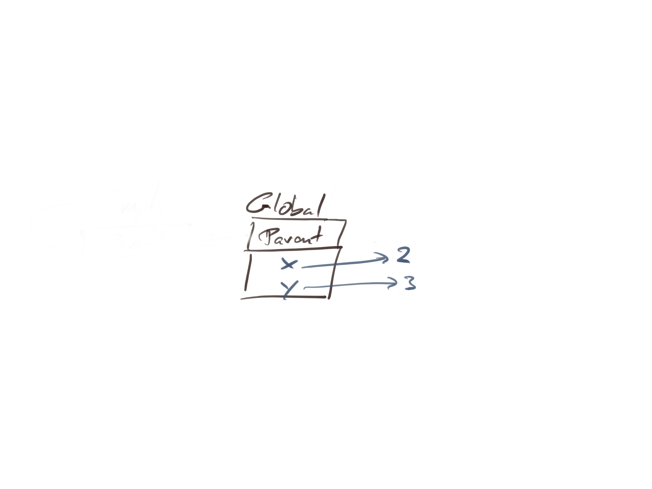
When you call ls() without arguments, you get the list of variables in the environment you are currently in. In this case, the global environment. You can also explicitly give ls() an environment. You get the global environment by calling the function globalenv():
ls(globalenv())
## [1] "x" "y"
Now, let’s define a function:
f <- function(x) x + y
We are really doing two things in this statement. We create a function
function(x) x + y
and we assign it to the variable f. The effect of the assignment is simple; we add f to the (global) environment and make it point to the function. The function definition is a bit more involved.
We don’t need to know all the gory details of how functions work, but we need to know that functions have associated environments. You can get these by calling the function environment() on them.
environment(f)
## <environment: R_GlobalEnv>
You can change this environment if you want to, but by default, it is the environment in which you defined the function. In this case, the global environment.
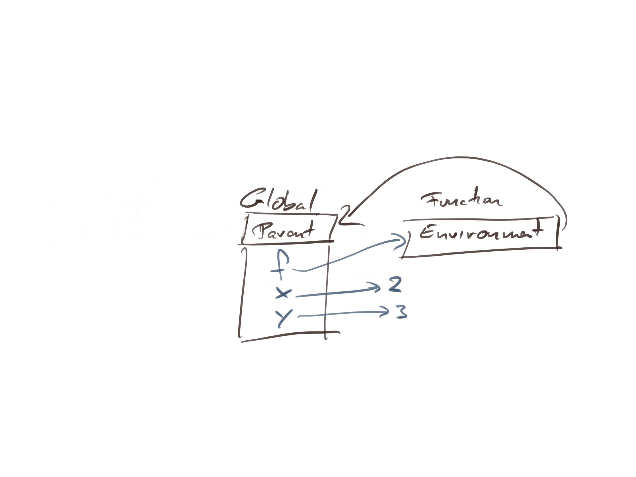
The function environment is not a new environment, however. You do not create an environment when you define a function. You just associate an environment with it. This environment is used as the parent of environments you create when you call a function.
If you call a function, e.g. call
f(5)
you will create a new environment. You put function arguments and local variables into this environment, and the parent of the environment is the environment associated with the function.
When you evaluate the x + y in the body of f, R will first check the function instance environment, where it will find x mapped to five, and then search up the parent chain for y, which it will find in the global environment mapped to three.
The combination of associating environments to functions and making these the parents of function-call environment enables you to get closures.
Get rid of x and y and define a function that nests another function
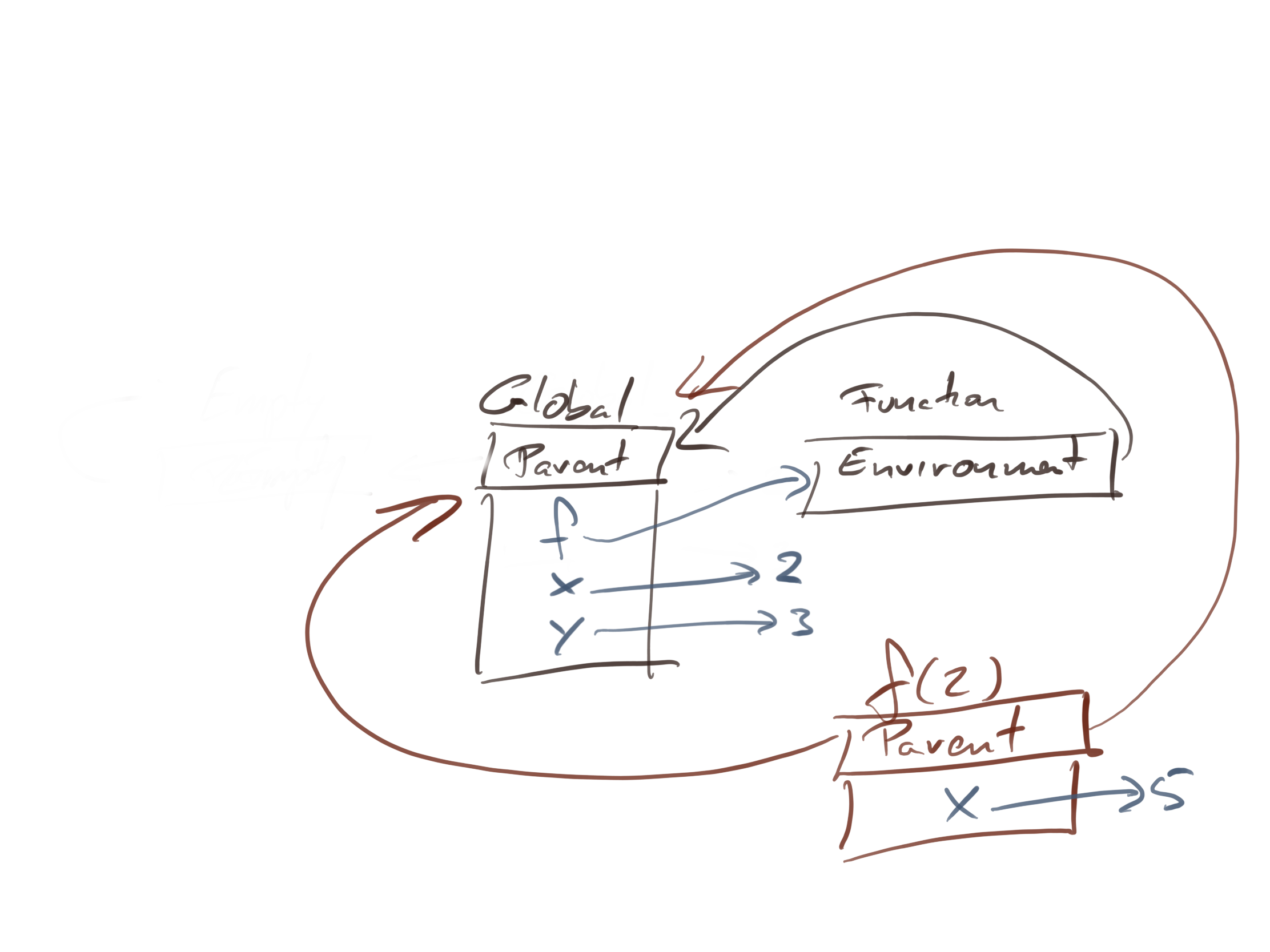
rm("x", "y")
f <- function(x) {
    g <- function(y) x + y
    g
}
After we have defined the function and assigned it to f, the global environment maps f to the function and the function’s environment is the global variable.
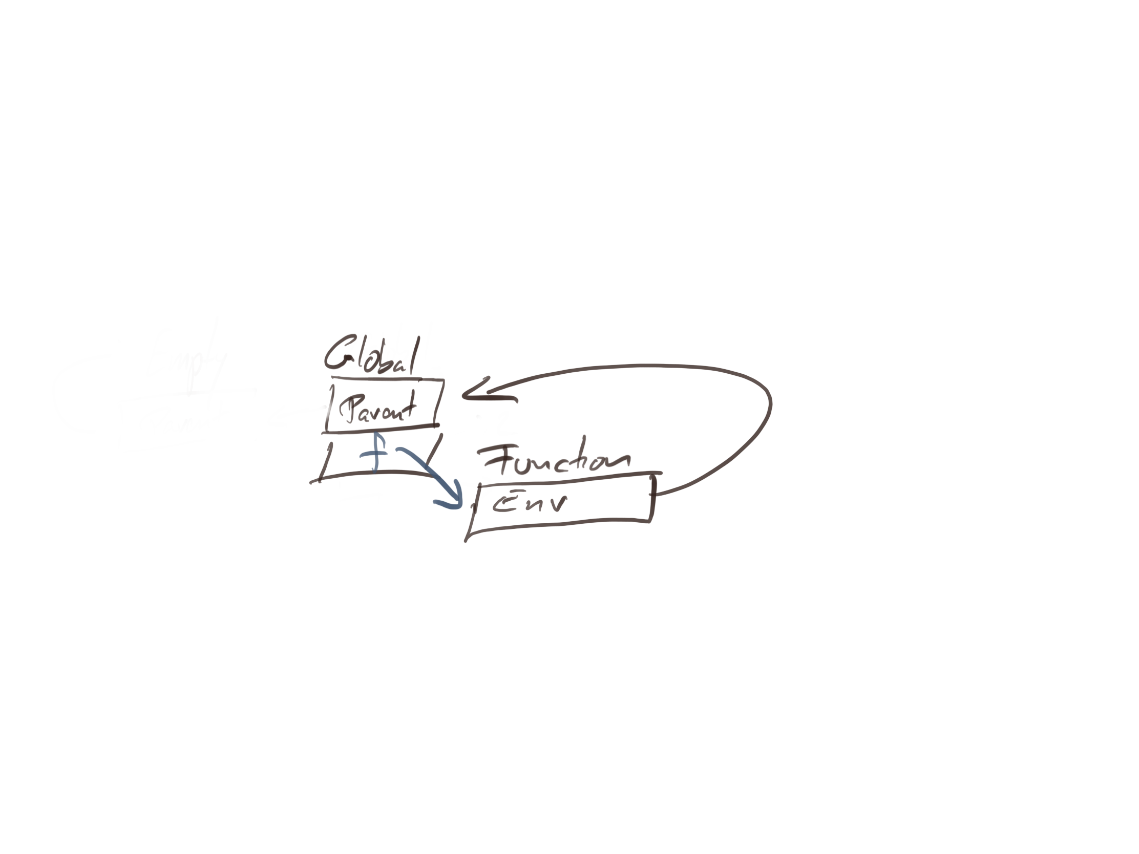
It doesn’t matter what happens inside the function body, because we haven’t evaluated it yet. There is no inner function yet; it doesn’t exist before we evaluate f.
Now, let us call f with argument 2. This creates an instance-environment and set its parent to the global environment (the environment of function f). Inside this environment, we store the argument x and the local function g. The environment of g is the instance environment of the f(2) call.
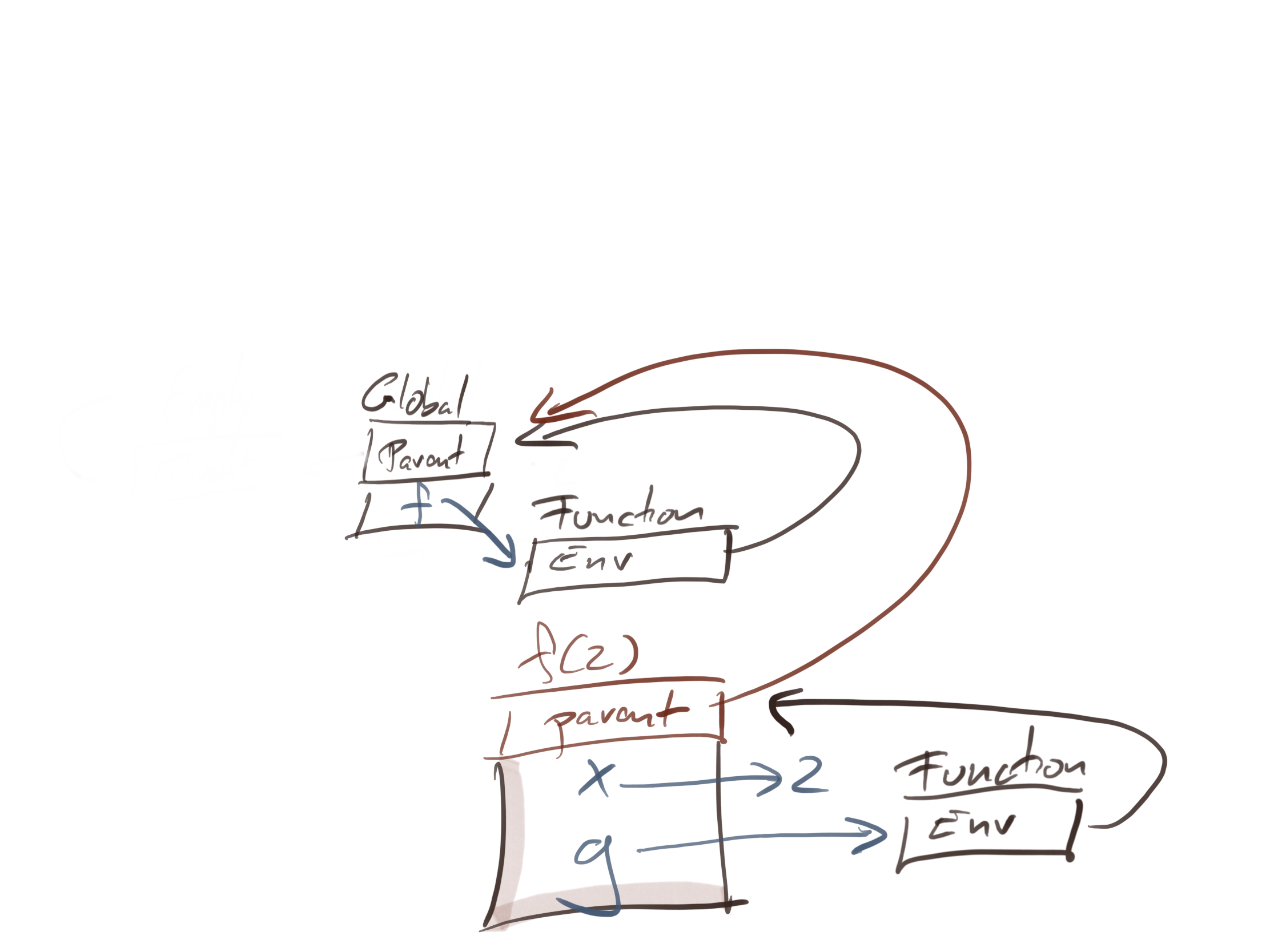
When you return from the call to f and assign the result to h, you have this setup:
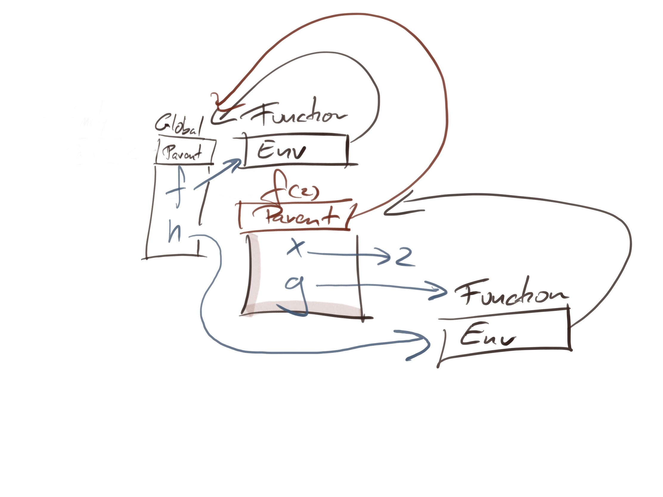
You do not have a direct handle on the instance-environment from the call to f, but it exists as the parent of the function environment of h.
If you then call h(3) you create another instance environment in which you map y to three. The parent environment is the function h’s environment—we are applying the same rule as before about instance environments and functions—so the state of the system in the call is this:
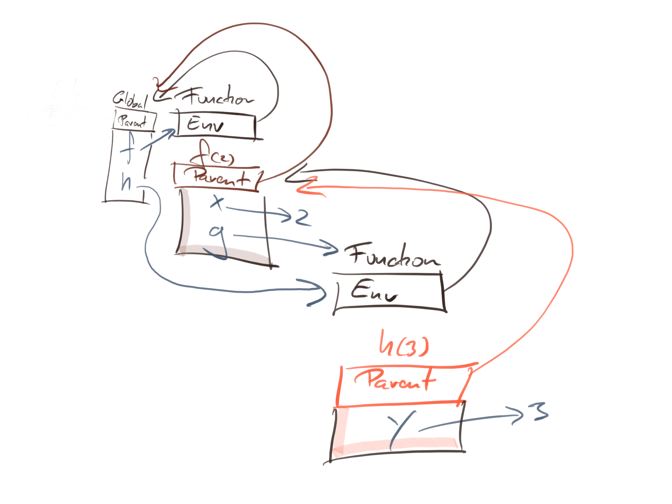
To evaluate x + y inside the h(3) call, we have this chain of environments:
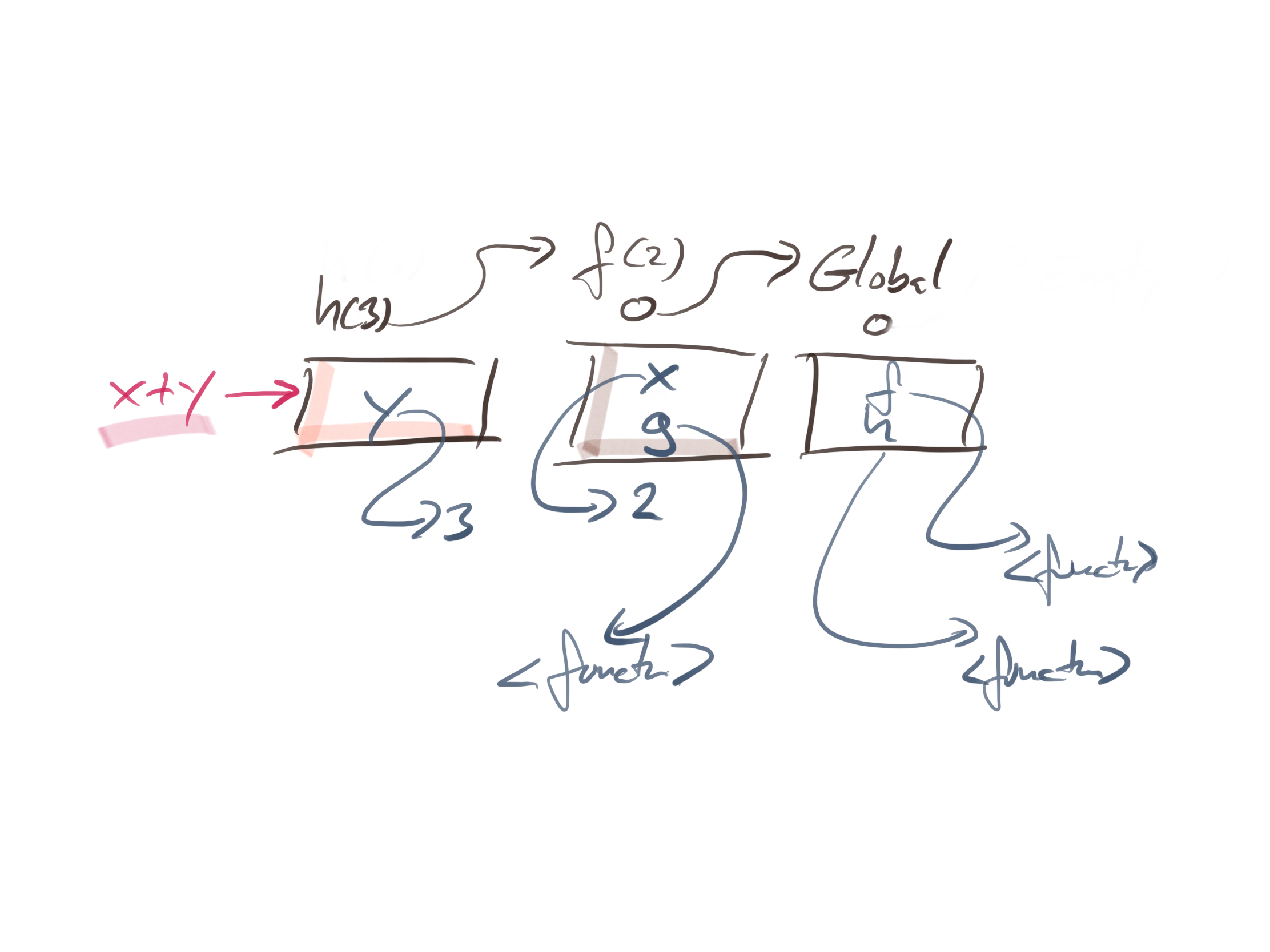
When we look for y, we can find it directly in the current environment. To find x we need to look in its parent. If we wanted f, g, and h we would find them in the chain as well.
If you have done any functional programming in R, this behaviour shouldn’t surprise you. It is lexical scope, and pretty much all modern languages have similar rules.
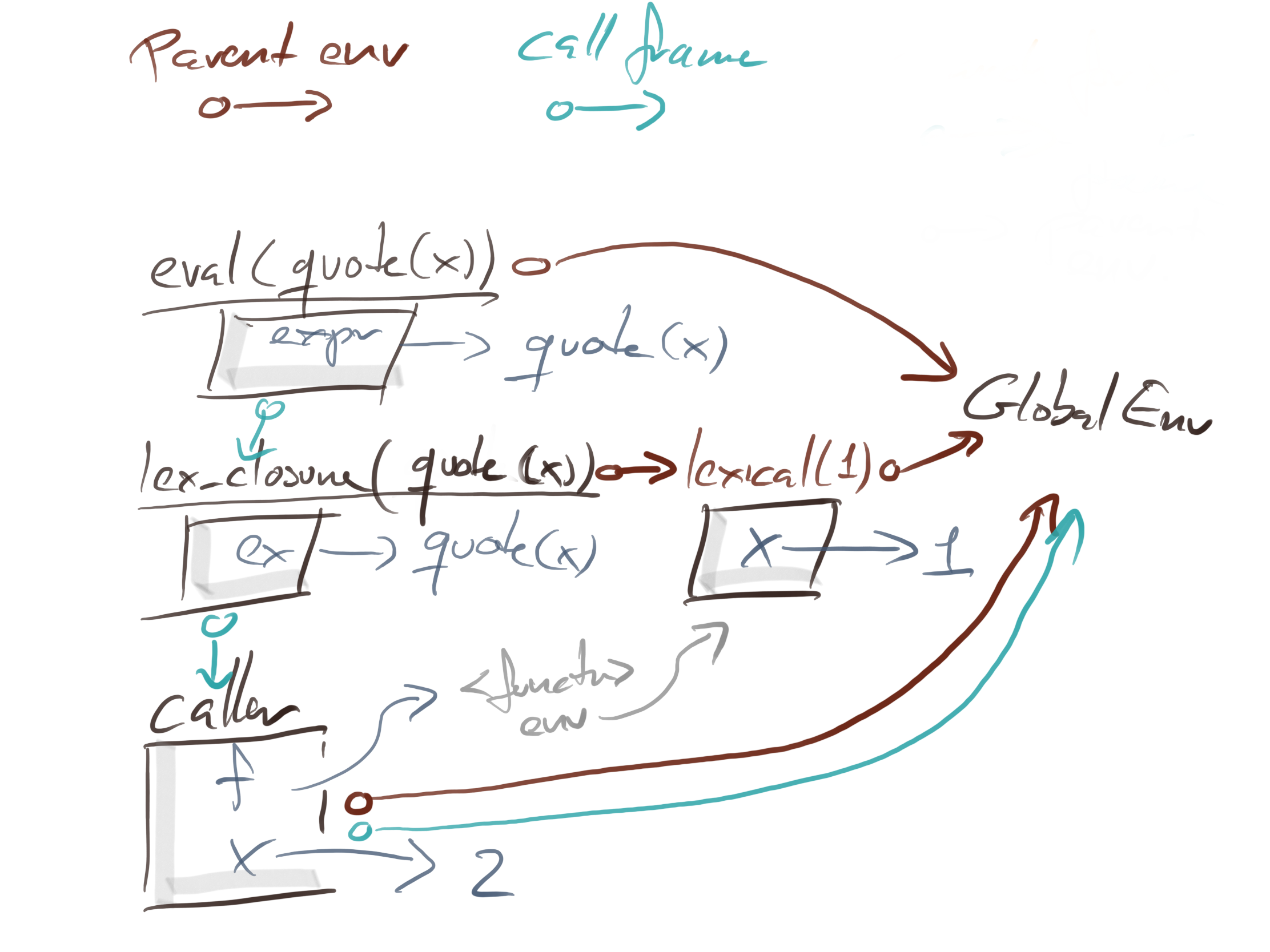
When we have quoted expressions added to the mix, we do not have to put the expression inside the nested function’s body. We can make it take an expression and evaluate it in its body. This separates where we define the (quoted) expression from where we evaluate it:
f <- function(x) function(y) function(ex) eval(substitute(ex))
g <- f(2)
h <- g(3)
h(x + y)
## [1] 5
h(x * y)
## [1] 6
Here, I use substitute to translate an argument into an expression. If you want to quote the arguments explicitly that is even simpler; I leave that as an exercise.
The expression we give the final nested function is evaluated in the scope of the innermost function. But how does eval know about that environment?
The parent environment of the eval call is the environment where we defined the eval function, which is the global environment.^[Actually, eval doesn’t live in the global environment, but as I said earlier, we simplify the discussion by pretending that the global environment is the root of all the environments. It doesn’t matter that it isn’t for the points I want to make in this post.] That environment doesn’t know anything about the variables we captured in the different closures when we constructed the function h.
When we call eval, we do not want it to evaluate its input in its own environment; rather, we want it to evaluate it in the caller’s environment.
Traditionally, we call function instances on the call stack frames. Since instance environment can survive longer than function calls, we are not really working with proper frames, but the terminology persists. We want to evaluate the expression we give eval in the caller’s frame, not in eval’s environment.
Well, eval is implemented using magic, and this is exactly what it does; it evaluates its input in the caller’s frame.^[When I say magic, I am not far from the truth. The eval function uses a function that is built into the R runtime system, and that means that it can do more than we can do with normal R functions. We cannot implement eval as a normal R function, because we need the functionality that eval provides to do that. Some magic is needed. Once we have it, though, we can exploit the hell out of it.]
We cannot write magical functions, but we can use eval to get the same effect. We can give eval a second argument, and it will use that as the environment to evaluate the expression in. We can get the caller’s environment, rather than our own, through the function parent.frame. This is an unusually poor choice of function name because the caller’s frame has nothing to do with parent environments, but that is what it is called. The function rlang::caller_env does the same, and it has a more sensible name.
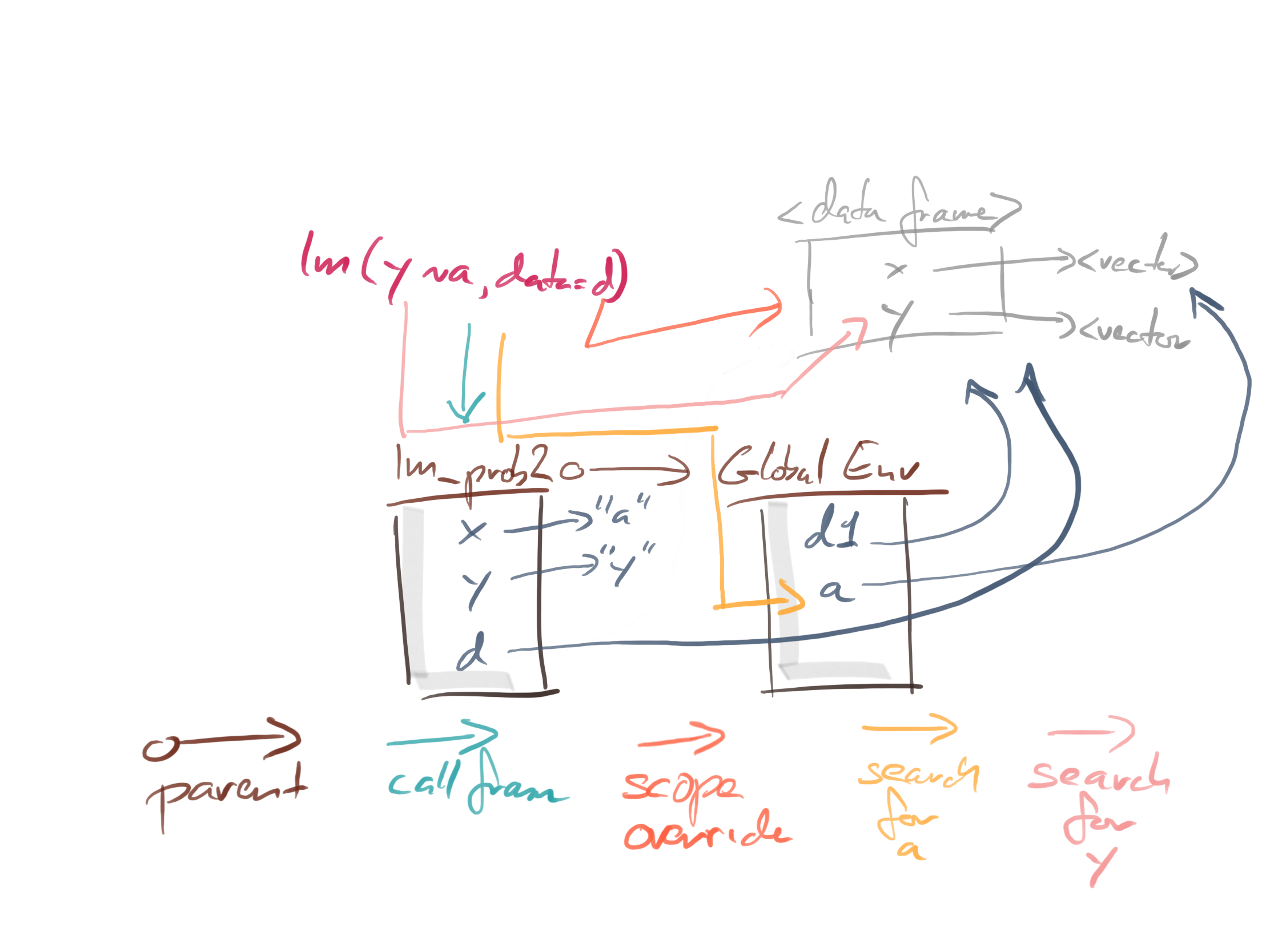
Consider this setup:
lexical <- function(x) function(ex) eval(ex)
dynamic <- function(x) function(ex) eval(ex, parent.frame())
lex_closure <- lexical(1)
dyn_closure <- dynamic(1)
Here, we have two functions that create closures, and we create one from each. I have called them lexical and dynamic because they implement lexical and dynamic scoping, respectively. Don’t worry about the terminology if it is unfamiliar. All sensible languages use lexical scoping—it is much easier to reason about—but dynamic scoping is something we can exploit in a non-standard evaluation. You will see the difference between the two in just a second.
After creation lex_closure and dyn_closures, the setup looks very similar.
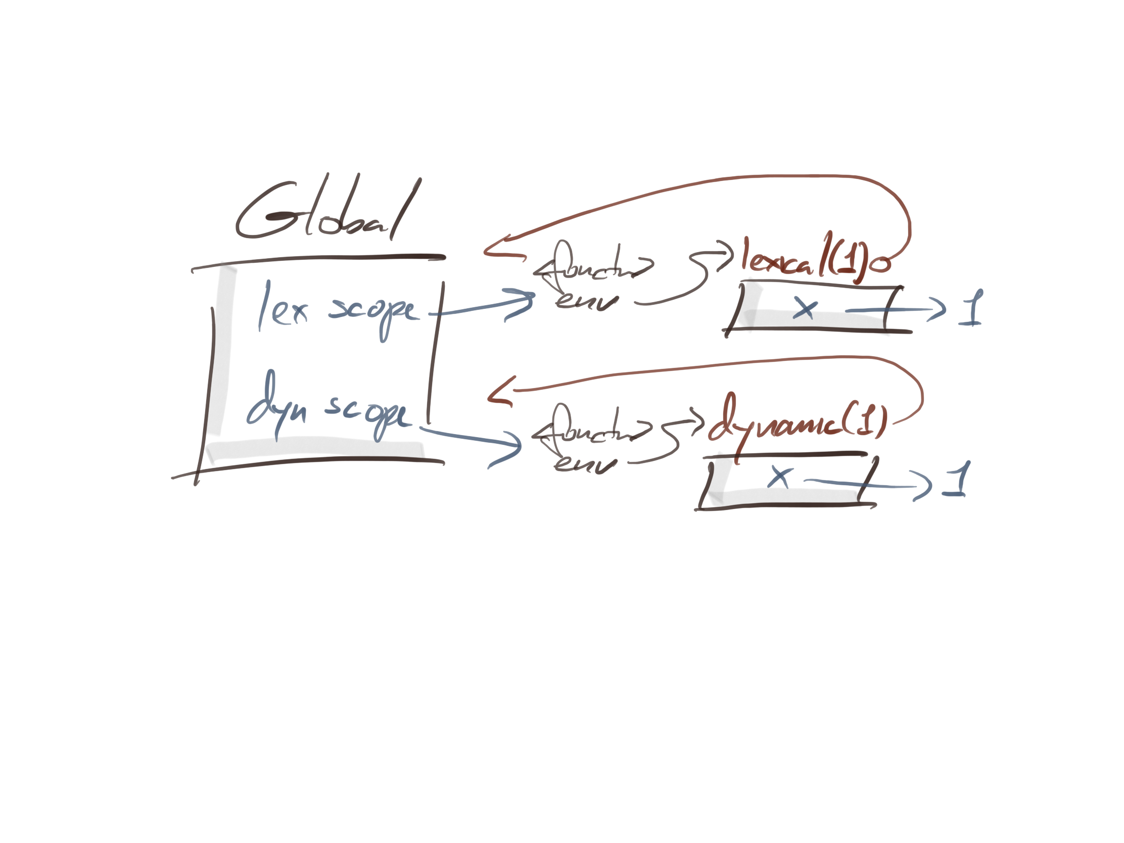
Both closures have an environment that contains a value for x—in both cases that value is 1—and both environments have the global environment as the parent. The only difference in the two closures is the function body we execute when we call them.
Try this:
caller <- function(x, f) f(quote(x))
caller(2, lex_closure)
## [1] 1
caller(2, dyn_closure)
## [1] 2
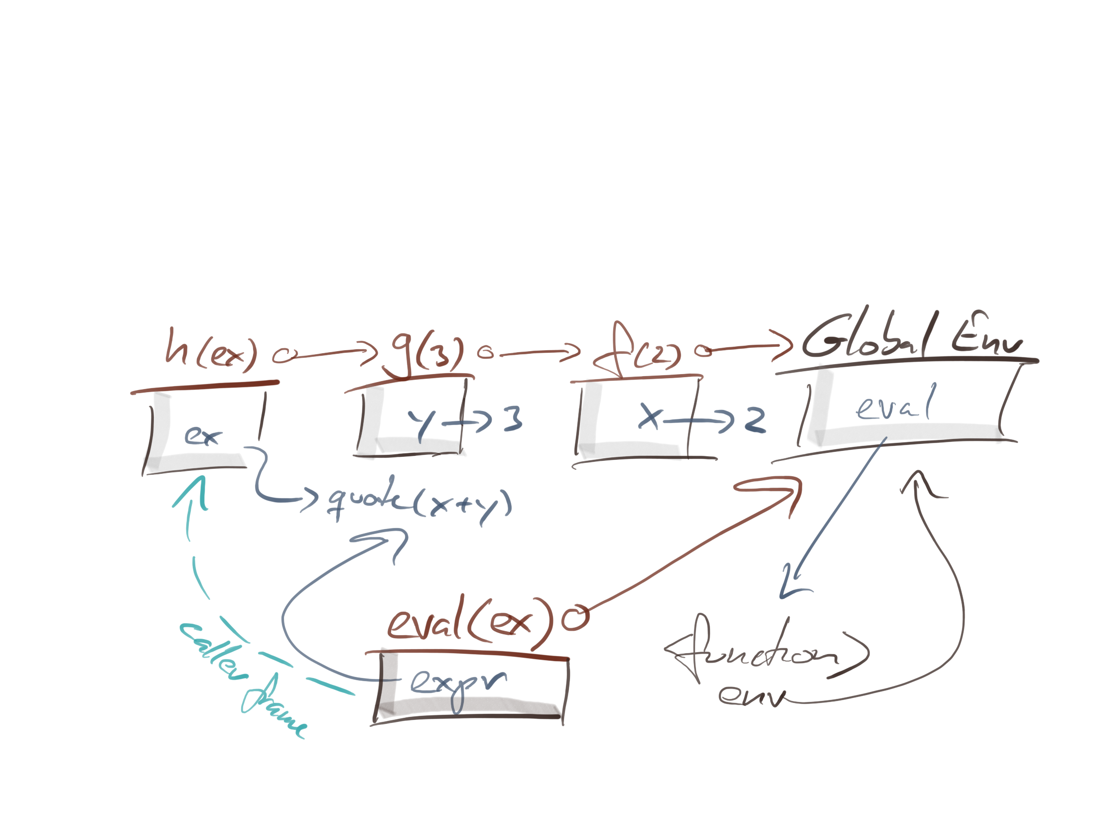
The two calls to caller look the same. You get this graph of function instances with parent environments (in brown) and caller frames (in blue) regardless of whether you use the lex closure or the dyn closure.
The difference between the two calls is the path that R takes to search for x. In the lexical scoping closures, eval will look in its caller frame, which is the lex_closure instance, and then search up the parent chain there.
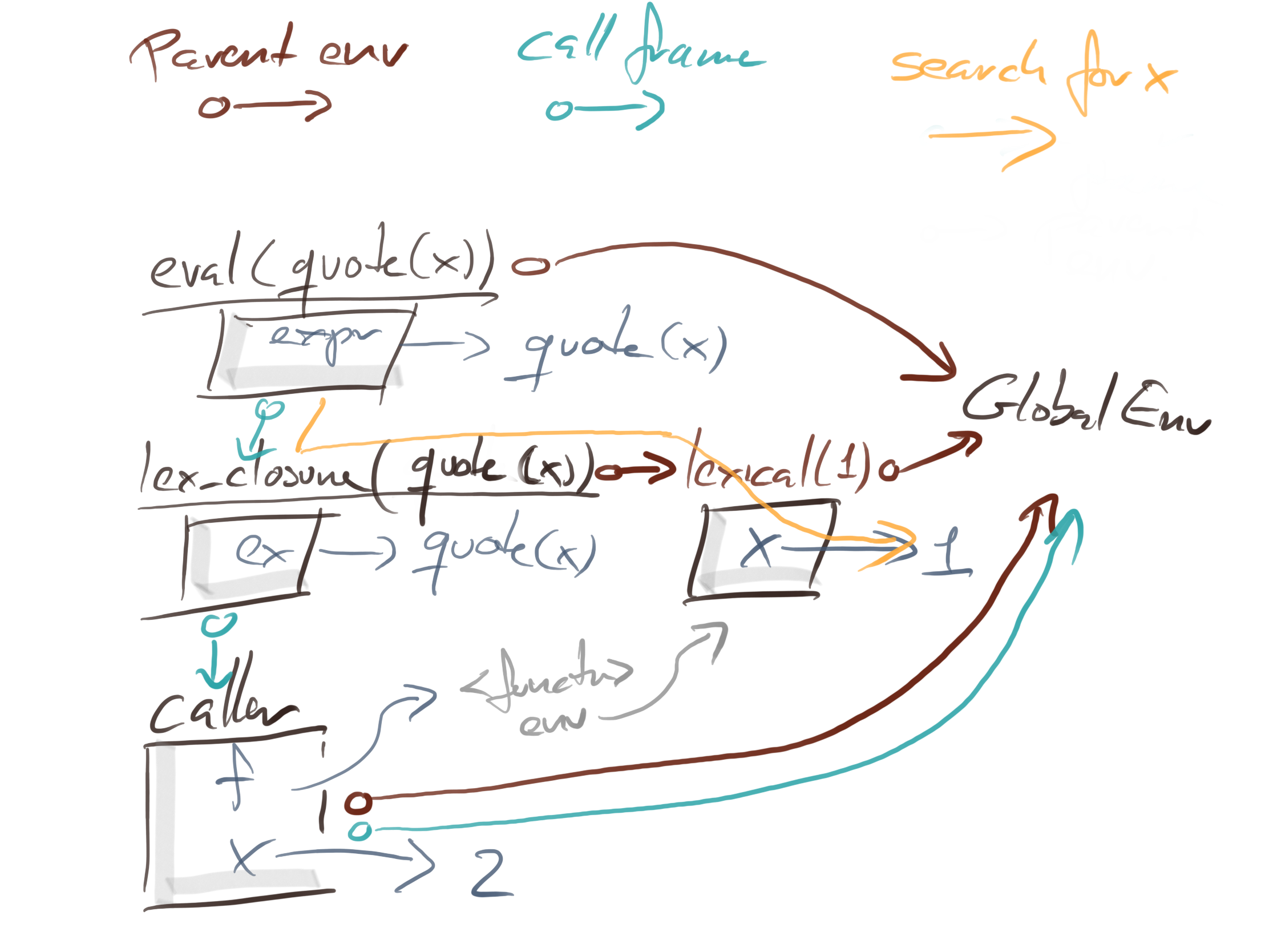
With dyn_closure we connect eval with dyn_closure’s calling frame, so we skip dyn_closure’s instance environment entirely and search in caller instead, where we find x.
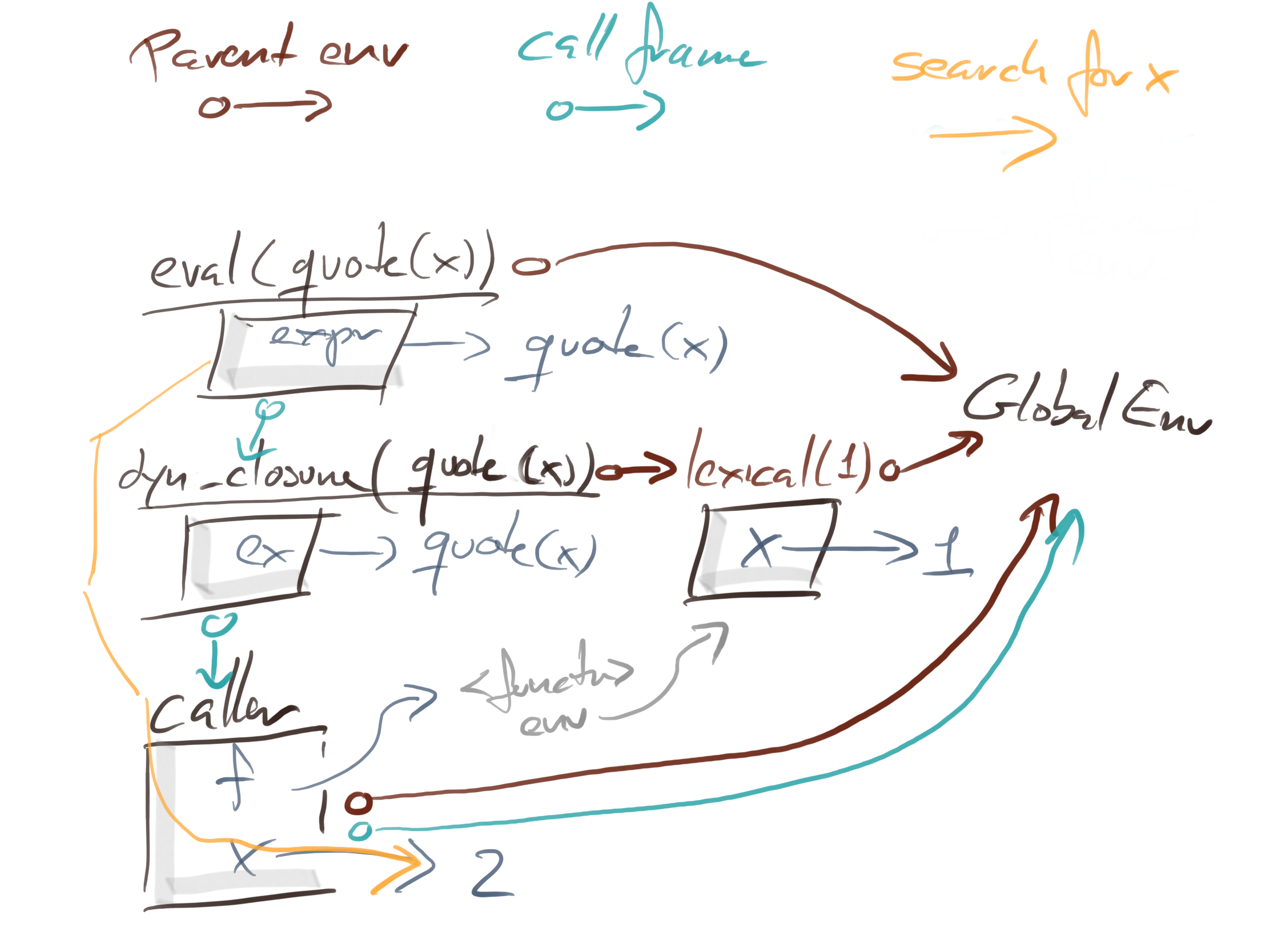
The figures are getting a bit crowded by now, but I am sure you can work your way through them, with little effort. They capture most of what you need to know about scopes and evaluation: how environments are chained together by the lexical scope and how function call-stacks are chained together through caller frames.
When you evaluate an expression, you always search for variable-value bindings in the chain of environment parents. Non-standard evaluation is all about starting the search somewhere you do not usually start it or constructing alternative parent-chains than those you would typically use.
There’s a bit more to the story. Functions are not the only objects that have environments attached to them. Promises and formulas and quosures (which are really formulas) have as well. There are also environment rules for packages, but to understand the actual language that is not so essential. There is also more to how eval finds values—it doesn’t just let you choose an alternative environment path, it also lets you find values in lists and data frames. All that must wait for another post; this one is getting long enough as it is.
In any case, to understand the tweets that I wrote a few days ago, the explanation above will suffice. I will repeat the examples from my tweets below. They use wrapr::let to substitute variables in expressions with values. This function works slightly different from substitute, so there are some differences, but you should easily be able to understand the examples. Maybe I will try to rewrite them using substitute in a later post.
Examples using wrapr::let
Ok, for the examples I imagined that I had some data frames, that I want to fit a linear model on the data, and that I then want to extract some property from the fitted model. The variables in the model depend on the data frame, though, and I might want to extract different properties.
So, I have this setup:
# Data:
d1 <- data.frame(x = rnorm(5), y = rnorm(5))
d2 <- data.frame(a = rnorm(5), b = rnorm(5))

# Not unreasonable usage:
summary(lm(y ~ x, data = d1))[["residuals"]]
##           1           2           3           4           5
##  0.04477841 -0.54955468 -0.68726607 -0.72583989  1.91788224
summary(lm(b ~ a, data = d2))[["residuals"]]
##          1          2          3          4          5
##  0.2206216 -0.9706430 -0.1337413  1.3052772 -0.4215145
The way formulas work in R, you can combine variables from data frames with variables known where you created the formula. In this case the global environment. So we can mix global variables with variables from the data frames like this:
xx <- rnorm(5)
summary(lm(y ~ xx, data = d1))[["residuals"]]
##          1          2          3          4          5
##  0.2662110 -1.4082401  0.1057206 -0.4657714  1.5020799
summary(lm(b ~ xx, data = d2))[["residuals"]]
##           1           2           3           4           5
## -0.01405177 -0.73169414 -0.49131556  1.47527203 -0.23821056
Now, I might want to parameterise these expressions in a function that looks like this:
lm_prop <- function(x, y, d, prop) {
    m <- lm(y ~ x, data = d)
    summary(m)[[prop]]
}
lm_prop(x, y, d1, "residuals")
##           1           2           3           4           5
##  0.04477841 -0.54955468 -0.68726607 -0.72583989  1.91788224
Great, this looks like it is working, but that is an unfortunate coincidence. It works because the data frame d1 contains variables x and y, and those happen to be the ones we want to fit. In the lm(y ~ x, data = d) call, however, the variables are quoted, so to speak. The formula is y ~ x, and we do not substitute x and y with the arguments to lm_prop.
Because of this, we get an error if we try to fit a model from d2:
lm_prop(a, b, d2, "residuals")
## Error in eval(predvars, data, env): objekt 'b' blev ikke fundet
To get this to work, we need to substitute arguments into the model-fitting.
The wrapr::let function works that way. It lets us substitute variables, and after the substitution, we can evaluate the expression. If the parameter eval is TRUE the expression will be evaluated; if it is FALSE, it will not.
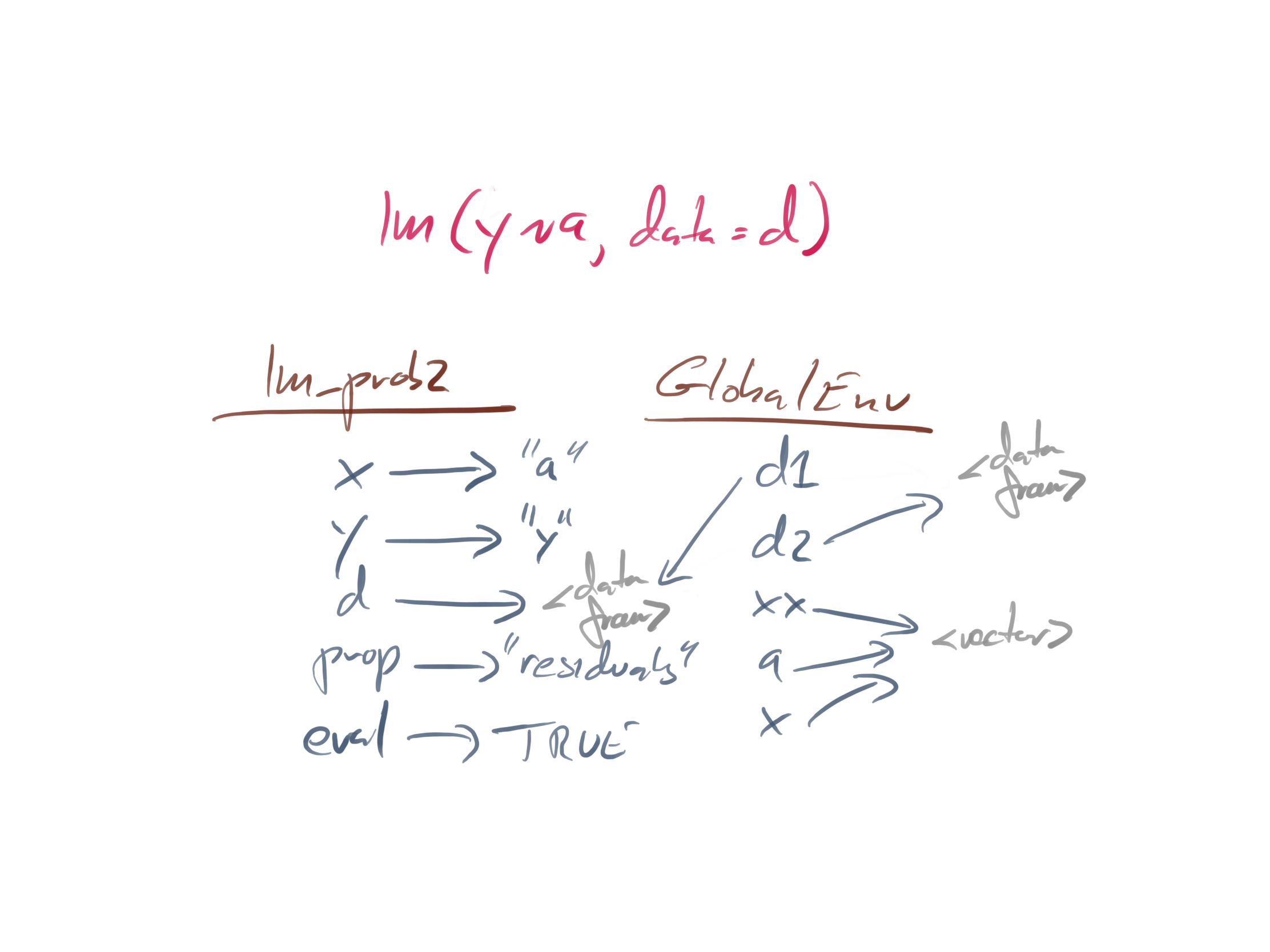
We can define our lm_prop function like this:
library(wrapr)
lm_prop2 <- function(x, y, d, prop, eval) {
    let(c(x = x, y = y, prop = prop),
        summary(lm(y ~ x, data = d))$prop,
        eval = eval)
}
We can check that it works:
# Data frame variables
lm_prop2("x", "y", d1, "residuals", eval = FALSE)
## summary(lm(y ~ x, data = d))$residuals
summary(lm(y ~ x, data = d1))$residuals
##           1           2           3           4           5
##  0.04477841 -0.54955468 -0.68726607 -0.72583989  1.91788224
lm_prop2("x", "y", d1, "residuals", eval = TRUE)
##           1           2           3           4           5
##  0.04477841 -0.54955468 -0.68726607 -0.72583989  1.91788224
# Mixed variables
lm_prop2("xx", "y", d1, "residuals", eval = FALSE)
## summary(lm(y ~ xx, data = d))$residuals
lm_prop2("xx", "y", d1, "residuals", eval = TRUE)
##          1          2          3          4          5
##  0.2662110 -1.4082401  0.1057206 -0.4657714  1.5020799
summary(lm(y ~ xx, data = d1))$residuals
##          1          2          3          4          5
##  0.2662110 -1.4082401  0.1057206 -0.4657714  1.5020799
# Data frame variables
lm_prop2("a", "b", d2, "residuals", eval = FALSE)
## summary(lm(b ~ a, data = d))$residuals
summary(lm(b ~ a, data = d2))$residuals
##          1          2          3          4          5
##  0.2206216 -0.9706430 -0.1337413  1.3052772 -0.4215145
lm_prop2("a", "b", d2, "residuals", eval = TRUE)
##          1          2          3          4          5
##  0.2206216 -0.9706430 -0.1337413  1.3052772 -0.4215145
# Mixed variables
lm_prop2("xx", "b", d2, "residuals", eval = FALSE)
## summary(lm(b ~ xx, data = d))$residuals
summary(lm(b ~ xx, data = d2))$residuals
##           1           2           3           4           5
## -0.01405177 -0.73169414 -0.49131556  1.47527203 -0.23821056
lm_prop2("xx", "b", d2, "residuals", eval = TRUE)
##           1           2           3           4           5
## -0.01405177 -0.73169414 -0.49131556  1.47527203 -0.23821056
Great, it looks like it is working.
Whenever your code looks like it is working, if you are using non-standard evaluation, it is time to figure out why it only looks that way.
Surprisingly often, we get fooled by scopes—which is why I spent so much time explaining them above. That is also happening here.
Consider what we are doing when we mix global variables with data frame variables. If a variable can be found in the data frame then we use it; otherwise, we find a global variable. Since a isn’t found in d1, and x isn’t found in d2 we should be able to rename xx.
x <- a <- xx
and still be able to mix a data frame with global variables.
lm_prop2("a", "y", d1, "residuals", eval = FALSE)
## summary(lm(y ~ a, data = d))$residuals
summary(lm(y ~ a, data = d1))$residuals
##          1          2          3          4          5
##  0.2662110 -1.4082401  0.1057206 -0.4657714  1.5020799
lm_prop2("a", "y", d1, "residuals", eval = TRUE)
##          1          2          3          4          5
##  0.2662110 -1.4082401  0.1057206 -0.4657714  1.5020799
Ok, so far it looks fine.
Now try this:
lm_prop2("x", "b", d2, "residuals", eval = FALSE)
## summary(lm(b ~ x, data = d))$residuals
summary(lm(b ~ x, data = d2))$residuals
##           1           2           3           4           5
## -0.01405177 -0.73169414 -0.49131556  1.47527203 -0.23821056
lm_prop2("x", "b", d2, "residuals", eval = TRUE)
## Error in model.frame.default(formula = b ~ x, data = d, drop.unused.levels = TRUE): variable lengths differ (found for 'x')
Wait, what? Why doesn’t it work with x for d2?
The let function does precisely what it is supposed to do with the substitution. The problem is when we evaluate the result.
The setup that works looks like this:
The one that fails looks like this:
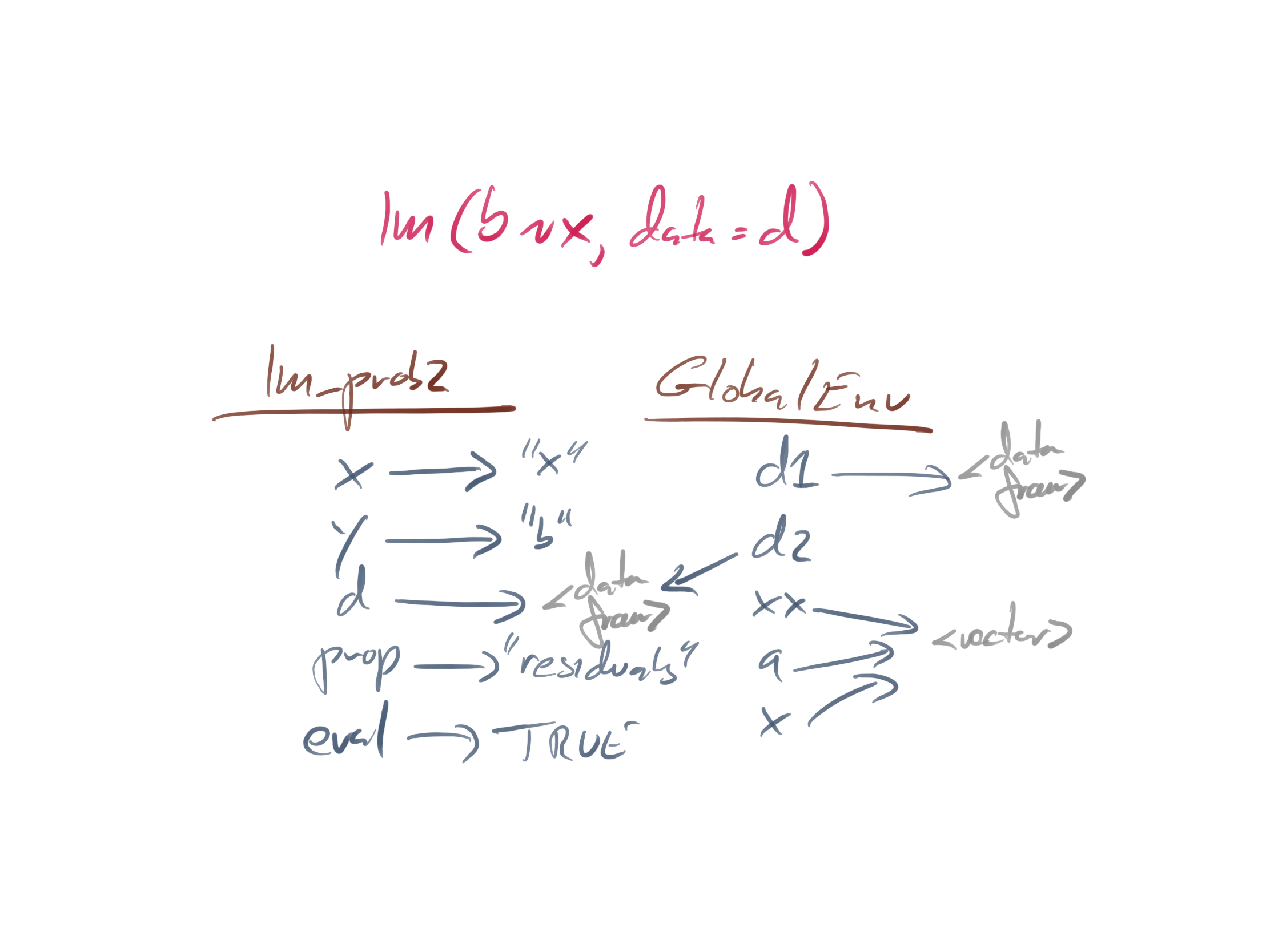
They look very similar, almost identically, so why does one work while the other does not?
The function lm also uses a non-standard evaluation. If we give it a data frame, it will look for variables there before it looks in the enclosing scope, i.e. the function that calls lm.
When we evaluate lm(y ~ a, data = d), we search for a and y like this:
When we evaluate lm(b ~ x, data = d), we search for x and b like this:
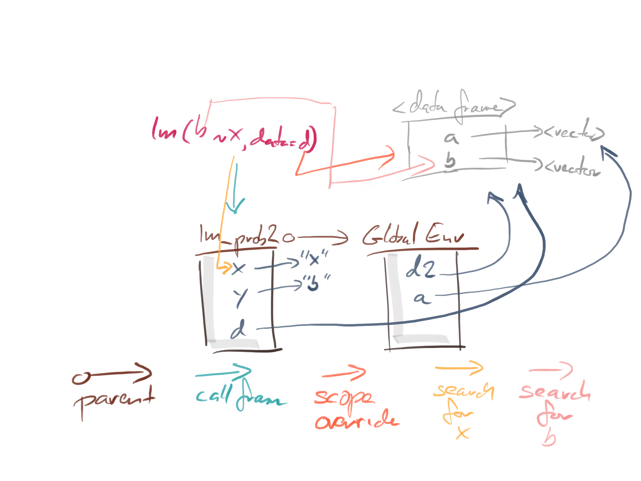
The x we find is the local variable, not the global one. That is why the function call fails.
For this function to work, you cannot have local variables that over-shadows global ones. You can fix the function like this:
lm_prop3 <- function(.a, .b, d, .prop, eval) {
    let(c(x = .a, y = .b, prop = .prop),
        summary(lm(y ~ x, data = d))$.prop,
        eval = eval)
}
lm_prop3("a", "y",  d1, "residuals", eval = FALSE)
## summary(lm(y ~ a, data = d))$.prop
summary(lm(y ~ a, data = d1))$residuals
##          1          2          3          4          5
##  0.2662110 -1.4082401  0.1057206 -0.4657714  1.5020799
lm_prop3("a", "y", d1, "residuals", eval = TRUE)
## NULL
lm_prop3("x", "b", d2, "residuals", eval = FALSE)
## summary(lm(b ~ x, data = d))$.prop
summary(lm(b ~ x, data = d2))$residuals
##           1           2           3           4           5
## -0.01405177 -0.73169414 -0.49131556  1.47527203 -0.23821056
lm_prop3("x", "b", d2, "residuals", eval = TRUE)
## NULL
This will work, I think.
But what if we had written the function in an almost identical way like this:
lm_prop4 <- function(.a, .b, .d, prop, eval) {
    let(c(x = .a, y = .b, d = .d, prop = prop),
        summary(lm(y ~ x, data = d))$prop,
        eval = eval)
}
lm_prop4("a", "y",  "d1", "residuals", eval = FALSE)
## summary(lm(y ~ a, data = d1))$residuals
summary(lm(y ~ a, data = d1))$residuals
##          1          2          3          4          5
##  0.2662110 -1.4082401  0.1057206 -0.4657714  1.5020799
lm_prop4("a", "y", "d1", "residuals", eval = TRUE)
##          1          2          3          4          5
##  0.2662110 -1.4082401  0.1057206 -0.4657714  1.5020799
lm_prop4("x", "b", "d2", "residuals", eval = FALSE)
## summary(lm(b ~ x, data = d2))$residuals
summary(lm(b ~ x, data = d2))$residuals
##           1           2           3           4           5
## -0.01405177 -0.73169414 -0.49131556  1.47527203 -0.23821056
lm_prop4("x", "b", "d2", "residuals", eval = TRUE)
##           1           2           3           4           5
## -0.01405177 -0.73169414 -0.49131556  1.47527203 -0.23821056
This looks like it is working. Can you spot where the problem is?
What happens if we call lm_prop4 from another function?
indirect <- function(xx, yy, eval) {
    d <- data.frame(x = xx, y = yy)
    lm_prop4("x", "y", "d", "residuals", eval = eval)
}

aa <- rnorm(5) ; bb <- rnorm(5)
summary(lm(bb ~ aa))$residuals
##          1          2          3          4          5
## -0.3157049 -0.1431962  0.7170060  0.2178049 -0.4759099
indirect(aa, bb, eval = FALSE)
## summary(lm(y ~ x, data = d))$residuals
indirect(aa, bb, eval = TRUE)
## Error in is.data.frame(data): objekt 'd' blev ikke fundet
It cannot find d because that name only exists in the call-environment of indirect(aa, bb, eval = TRUE).
The search for d goes as follows:
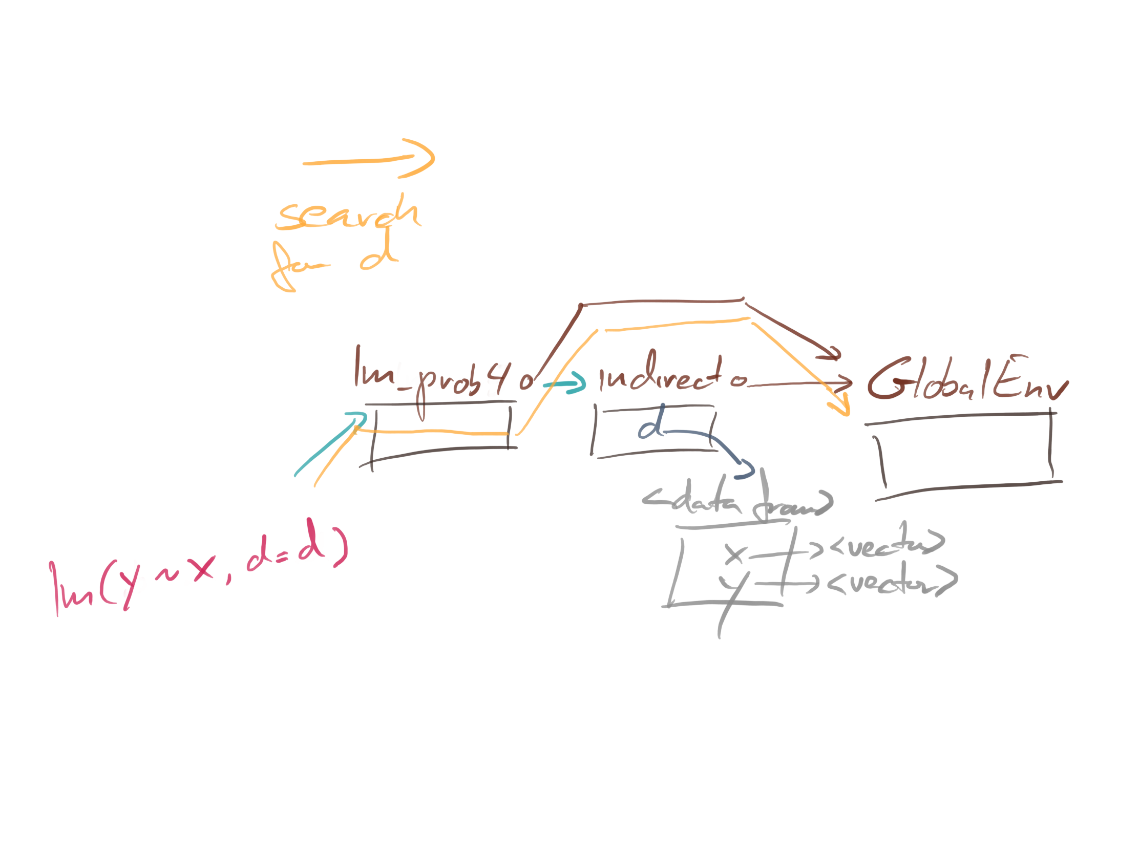
We do not follow the “caller frame” reference from lm_prob4 to indirect. We do get an error; we would be worse off if the global scope had a data frame called d. Then we might not get an error but instead just get the wrong result. That can be hard to debug.
If you want to fix the example, you can easily do so. You can give the let function an environment in which to evaluate the expression. If you do that, however, you cannot see the local variables in the function that calls let; it will look in the environment you give it instead of the caller frame.
It isn’t hard to change the current environment’s parent, and you can use that to chain the environment inside lm_prop4 and its caller, but then you lose the enclosing scope of lm_prop4—that scope is found through the parent chain, and you have just changed that.
It is not entirely impossible to get values both from the enclosing scope—through the parent pointer—as well as the calling scope. There are more environments around than those I have described here, and you can exploit that. I might explain that in another post. I explain it, in some detail, in my domain-specific language book, so you can always check it out there.
The take-home message of this post is not to pick on wrapr::let. It does what it says it does. I just think it is problematic with quick fixes for non-standard evaluation. If it looks easy, you might think it is. Worse, you might attempt to use it.
If you do not explicitly worry about scopes, non-standard evaluation can get very complicated very quickly. If you are lucky, you will get crash-errors, but you can also very easily just get the wrong result. If you do not spot that, you can be in a lot of trouble.
Non-standard evaluation is a powerful tool, but powerful tools should be handled with care.
-
I don’t like the term macro here, because to me it sounds like something that would happen at compile time (which in R would be when you translate code into bytecode). This doesn’t happen. There is no way (that I am aware of) to implement your own syntactic sugar that doesn’t involve evaluating code at runtime. ↩︎